Measurement error in models using SIMEX

Implementation of the SIMEX algorithm for measurement error models according to Cook and Stefanski

simex(model, SIMEXvariable, measurement.error, lambda = c(0.5, 1, 1.5,
  2), B = 100, fitting.method = "quadratic",
  jackknife.estimation = "quadratic", asymptotic = TRUE)

# S3 method for simex
plot(x, xlab = expression((1 + lambda)),
  ylab = colnames(b[, -1]), ask = FALSE, show = rep(TRUE, NCOL(b) -
  1), ...)

# S3 method for simex
predict(object, newdata, ...)

# S3 method for simex
print(x, digits = max(3, getOption("digits") - 3), ...)

# S3 method for summary.simex
print(x, digits = max(3, getOption("digits") -
  3), ...)

# S3 method for simex
refit(object, fitting.method = "quadratic",
  jackknife.estimation = "quadratic", asymptotic = TRUE, ...)

# S3 method for simex
summary(object, ...)

Arguments

model	the naive model
SIMEXvariable	character or vector of characters containing the names of the variables with measurement error
measurement.error	given standard deviations of measurement errors. In case of homoskedastic measurement error it is a matrix with dimension 1x`length(SIMEXvariable)`. In case of heteroskedastic error for at least one SIMEXvariable it is a matrix of dimension nx
lambda	vector of lambdas for which the simulation step should be done (without 0)
B	number of iterations for each lambda
fitting.method	fitting method for the extrapolation. `linear`, `quadratic`, `nonlinear` are implemented. (first 4 letters are enough)
jackknife.estimation	specifying the extrapolation method for jackknife variance estimation. Can be set to `FALSE` if it should not be performed
asymptotic	logical, indicating if asymptotic variance estimation should be done, in the naive model the option `x = TRUE` has to be set
x	object of class 'simex'
xlab	optional name for the X-Axis
ylab	vector containing the names for the Y-Axis
ask	logical. If `TRUE`, the user is asked for input, before a new figure is drawn
show	vector of logicals indicating for wich variables a plot should be produced
…	arguments passed to other functions
object	of class 'simex'
newdata	optionally, a data frame in which to look for variables with which to predict. If omitted, the fitted linear predictors are used
digits	number of digits to be printed

Value

An object of class 'simex' which contains:

coefficients

the corrected coefficients of the SIMEX model,

SIMEX.estimates

the estimates for every lambda,

model

the naive model,

measurement.error

the known error standard deviations,

the number of iterations,

extrapolation

the model object of the extrapolation step,

fitting.method

the fitting method used in the extrapolation step,

residuals

the residuals of the main model,

fitted.values

the fitted values of the main model,

call

the function call,

variance.jackknife

the jackknife variance estimate,

extrapolation.variance

the model object of the variance extrapolation,

variance.jackknife.lambda

the data set for the extrapolation,

variance.asymptotic

the asymptotic variance estimates,

theta

the estimates for every B and lambda,

...

Details

Nonlinear is implemented as described in Cook and Stefanski, but is numerically instable. It is not advisable to use this feature. If a nonlinear extrapolation is desired please use the refit() method.

Asymptotic is only implemented for naive models of class lm or glm with homoscedastic measurement error.

refit() refits the object with a different extrapolation function.

Methods (by generic)

plot: Plot the simulation and extrapolation step
predict: Predict using simex correction
print: Print simex nicely
print: Print summary nicely
refit: Refits the model with a different extrapolation function
summary: Summary of simulation and extrapolation

References

Cook, J.R. and Stefanski, L.A. (1994) Simulation-extrapolation estimation in parametric measurement error models. Journal of the American Statistical Association, 89, 1314 -- 1328

Carroll, R.J., Küchenhoff, H., Lombard, F. and Stefanski L.A. (1996) Asymptotics for the SIMEX estimator in nonlinear measurement error models. Journal of the American Statistical Association, 91, 242 -- 250

Carrol, R.J., Ruppert, D., Stefanski, L.A. and Crainiceanu, C. (2006). Measurement error in nonlinear models: A modern perspective., Second Edition. London: Chapman and Hall.

Lederer, W. and Küchenhoff, H. (2006) A short introduction to the SIMEX and MCSIMEX. R News, 6(4), 26--31

Examples

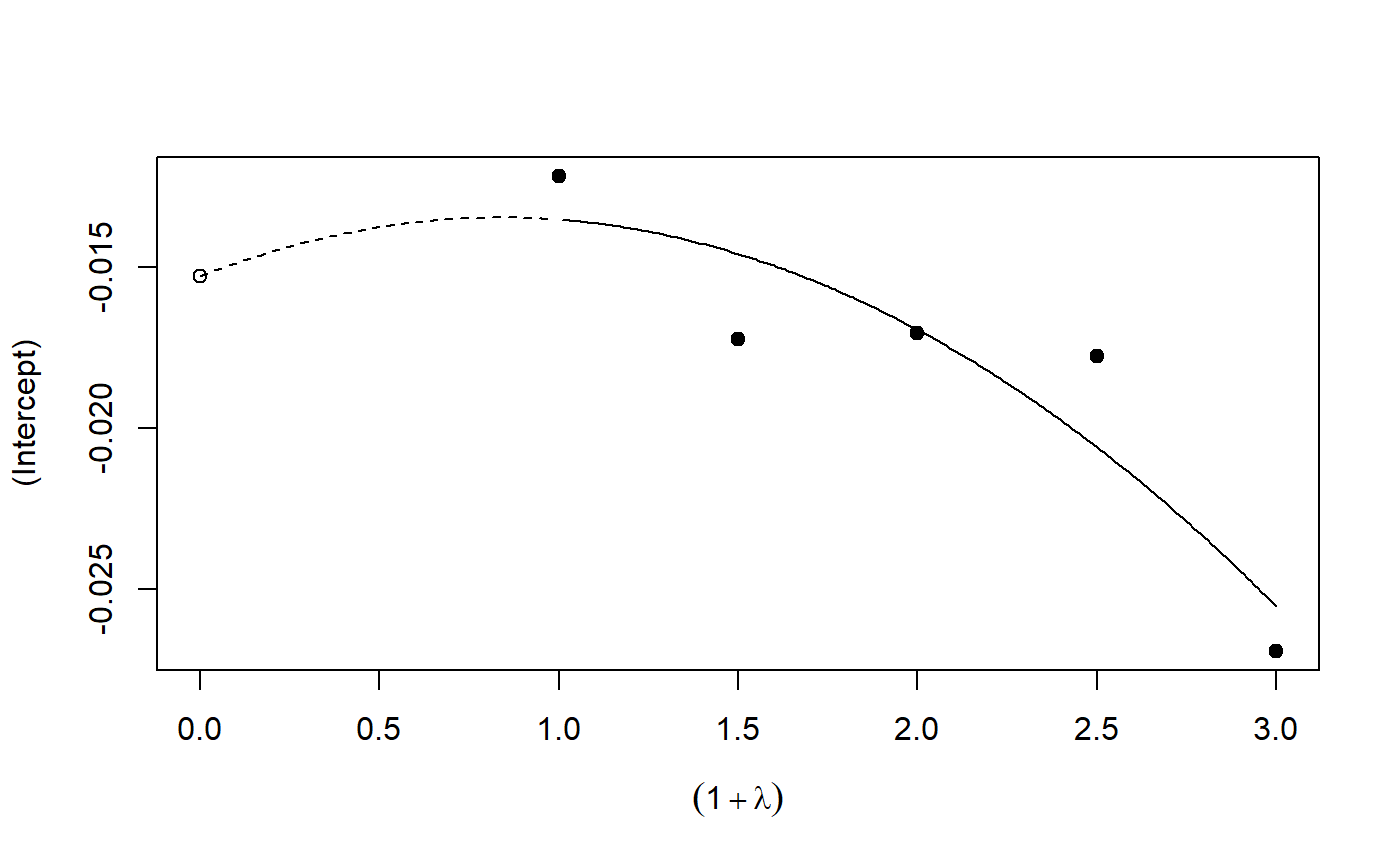
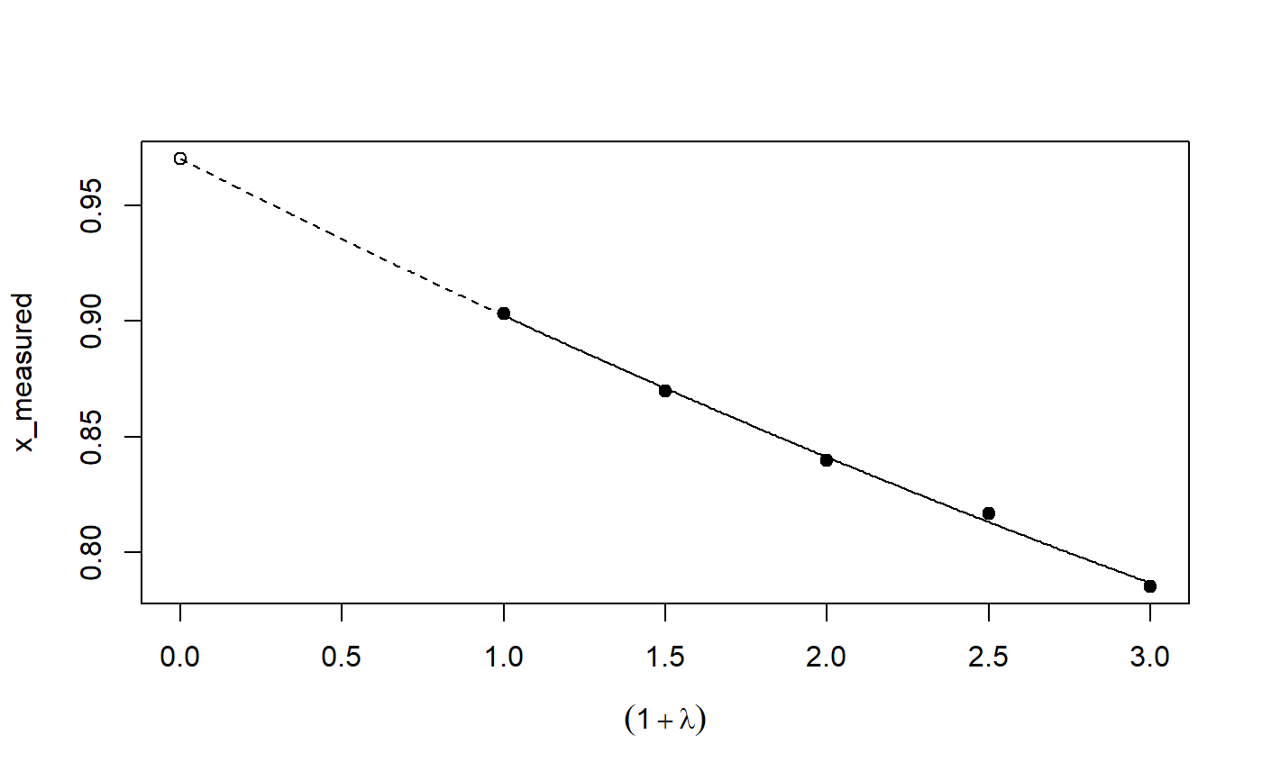
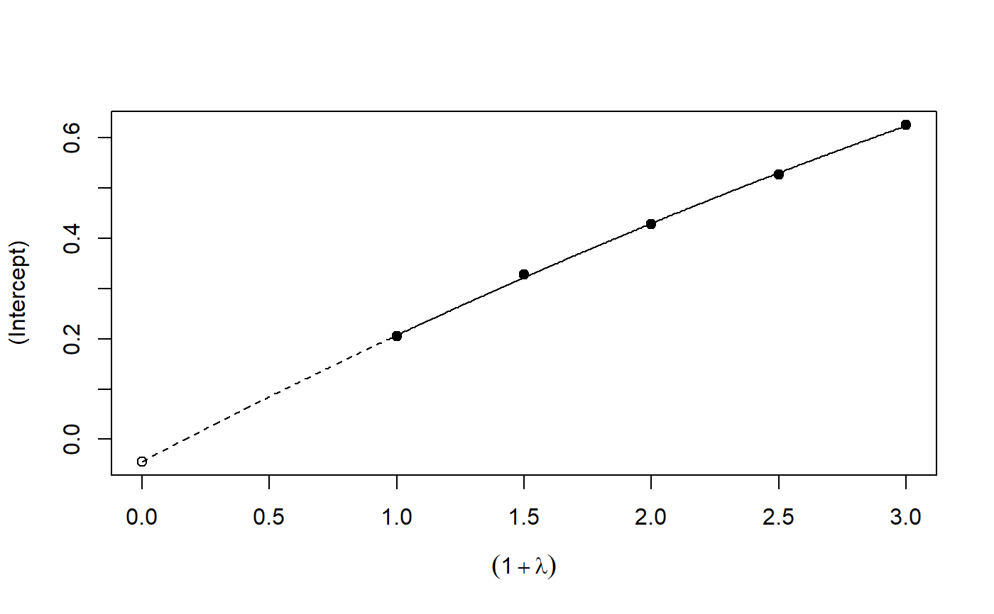
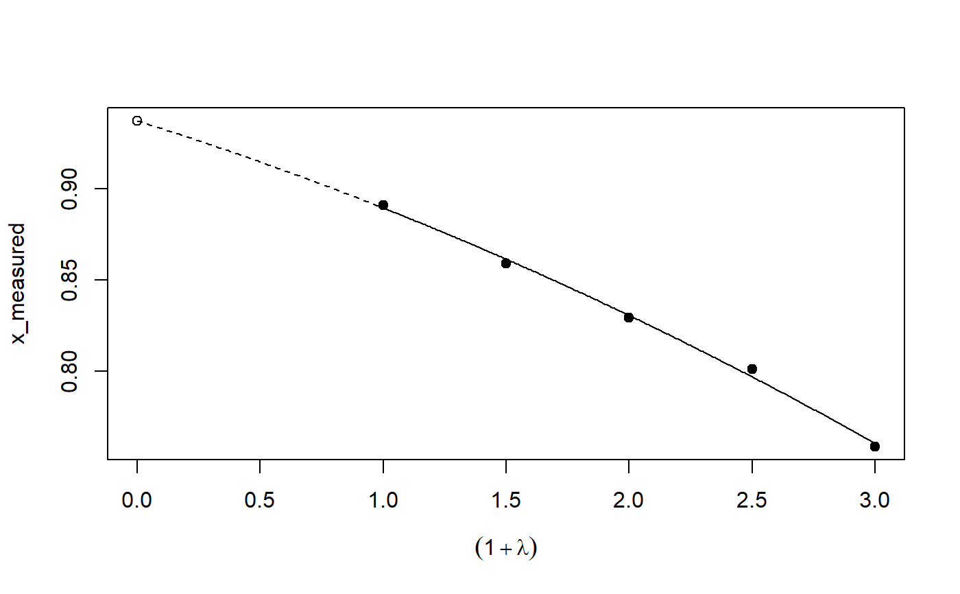
## Seed
set.seed(49494)

## simulating the measurement error standard deviations
sd_me <- 0.3
sd_me2 <- 0.4
temp <- runif(100, min = 0, max = 0.6)
sd_me_het1 <- sort(temp)
temp2 <- rnorm(100, sd = 0.1)
sd_me_het2 <- abs(sd_me_het1 + temp2)

## simulating the independent variables x (real and with measurement error):

x_real <- rnorm(100)
x_real2 <- rpois(100, lambda = 2)
x_real3 <- -4*x_real + runif(100, min = -10, max = 10)  # correlated to x_real

x_measured <- x_real + sd_me * rnorm(100)
x_measured2 <- x_real2 + sd_me2 * rnorm(100)
x_het1 <- x_real + sd_me_het1 * rnorm(100)
x_het2 <- x_real3 + sd_me_het2 * rnorm(100)

## calculating dependent variable y:
y <- x_real + rnorm(100, sd = 0.05)
y2 <- x_real + 2*x_real2 + rnorm(100, sd = 0.08)
y3 <- x_real + 2*x_real3 + rnorm(100, sd = 0.08)

### one variable with homoscedastic measurement error
(model_real <- lm(y ~ x_real))
#> 
#> Call:
#> lm(formula = y ~ x_real)
#> 
#> Coefficients:
#> (Intercept)       x_real  
#>   -0.004752     0.994554  
#> 

(model_naiv <- lm(y ~ x_measured, x = TRUE))
#> 
#> Call:
#> lm(formula = y ~ x_measured, x = TRUE)
#> 
#> Coefficients:
#> (Intercept)   x_measured  
#>    -0.01217      0.90327  
#> 

(model_simex <- simex(model_naiv, SIMEXvariable = "x_measured", measurement.error = sd_me))
#> 
#> Naive model:
#> lm(formula = y ~ x_measured, x = TRUE)
#> 
#> SIMEX-Variables: x_measured
#> Number of Simulations: 100
#> 
#> Coefficients:
#> (Intercept)   x_measured  
#>    -0.01528      0.97007  
#> 
plot(model_simex)

### two variables with homoscedastic measurement errors
(model_real2 <- lm(y2 ~ x_real + x_real2))
#> 
#> Call:
#> lm(formula = y2 ~ x_real + x_real2)
#> 
#> Coefficients:
#> (Intercept)       x_real      x_real2  
#>    -0.01411      0.99094      2.00011  
#> 
(model_naiv2 <- lm(y2 ~ x_measured + x_measured2, x = TRUE))
#> 
#> Call:
#> lm(formula = y2 ~ x_measured + x_measured2, x = TRUE)
#> 
#> Coefficients:
#> (Intercept)   x_measured  x_measured2  
#>      0.2050       0.8909       1.8593  
#> 
(model_simex2 <- simex(model_naiv2, SIMEXvariable = c("x_measured", "x_measured2"),
         measurement.error = cbind(sd_me, sd_me2)))
#> 
#> Naive model:
#> lm(formula = y2 ~ x_measured + x_measured2, x = TRUE)
#> 
#> SIMEX-Variables: x_measured, x_measured2
#> Number of Simulations: 100
#> 
#> Coefficients:
#> (Intercept)   x_measured  x_measured2  
#>    -0.04414      0.93716      1.97311  
#> 

plot(model_simex2)

# NOT RUN {
### one variable with increasing heteroscedastic measurement error
model_real

(mod_naiv1 <- lm(y ~ x_het1, x = TRUE))
(mod_simex1 <- simex(mod_naiv1, SIMEXvariable = "x_het1",
                measurement.error = sd_me_het1, asymptotic = FALSE))

plot(mod_simex1)

### two correlated variables with heteroscedastic measurement errors
(model_real3 <- lm(y3 ~ x_real + x_real3))
(mod_naiv2 <- lm(y3 ~ x_het1 + x_het2, x = TRUE))
(mod_simex2 <- simex(mod_naiv2, SIMEXvariable = c("x_het1", "x_het2"),
              measurement.error = cbind(sd_me_het1, sd_me_het2), asymptotic = FALSE))

plot(mod_simex2)

### two variables, one with homoscedastic, one with heteroscedastic measurement error
model_real2
(mod_naiv3 <- lm(y2 ~ x_measured + x_het2, x = TRUE))
(mod_simex3 <- simex(mod_naiv3, SIMEXvariable = c("x_measured", "x_het2"),
                    measurement.error = cbind(sd_me, sd_me_het2), asymptotic = FALSE))

### glm: two variables, one with homoscedastic, one with heteroscedastic measurement error
t <- x_real + 2*x_real2 + rnorm(100, sd = 0.01)
g <- 1 / (1 + exp(t))
u <- runif(100)
ybin <- as.numeric(u < g)

(logit_real <- glm(ybin ~ x_real + x_real2, family = binomial))
(logit_naiv <- glm(ybin ~ x_measured + x_het2, x = TRUE, family = binomial))
(logit_simex <- simex(logit_naiv, SIMEXvariable = c("x_measured", "x_het2"),
                    measurement.error = cbind(sd_me, sd_me_het2), asymptotic = FALSE))

summary(logit_simex)
print(logit_simex)
plot(logit_simex)

### polr: two variables, one with homoscedastic, one with heteroscedastic measurement error

if(require("MASS")) {# Requires MASS
yerr <- jitter(y, amount=1)
yfactor <- cut(yerr, 3, ordered_result=TRUE)

(polr_real <- polr(yfactor ~ x_real + x_real2))
(polr_naiv <- polr(yfactor ~ x_measured + x_het2, Hess = TRUE))
(polr_simex <- simex(polr_naiv, SIMEXvariable = c("x_measured", "x_het2"),
                    measurement.error = cbind(sd_me, sd_me_het2), asymptotic = FALSE))

summary(polr_simex)
print(polr_simex)
plot(polr_simex)
}
# }