Error or misclassification correction in models using (MC)SIMEX

Package simex is an implementation of the SIMEX--algorithm by Cook and Stephanski and the MCSIMEX--Algorithm by Küchenhoff, Mwalili and Lesaffre.

Details

	Package:
simex
Type:	Package
	Version:
1.8
Date:	2019-07-28
	License:
GPL 2 or above
LazyLoad:	yes

The package includes first of all the implementation for the SIMEX-- and MCSIMEX--Algorithms. Jackknife and asymptotic variance estimation are implemented. Various methods and analytic tools are provided for a simple and fast access to the SIMEX-- and MCSIMEX--Algorithm.

Functions simex() and mcsimex() can be used on models issued from lm(), glm() with asymtotic estimation. Models from nls(), gam() (package mgcv), polr() (package MASS), lme(), nlme() (package nlme) and coxph() (package survival) can also be corrected with these algorithms, but without asymptotic estimations.

References

Lederer, W. and Küchenhoff, H. (2006) A short introduction to the SIMEX and MCSIMEX. R News, 6/4, 26 -- 31

Examples

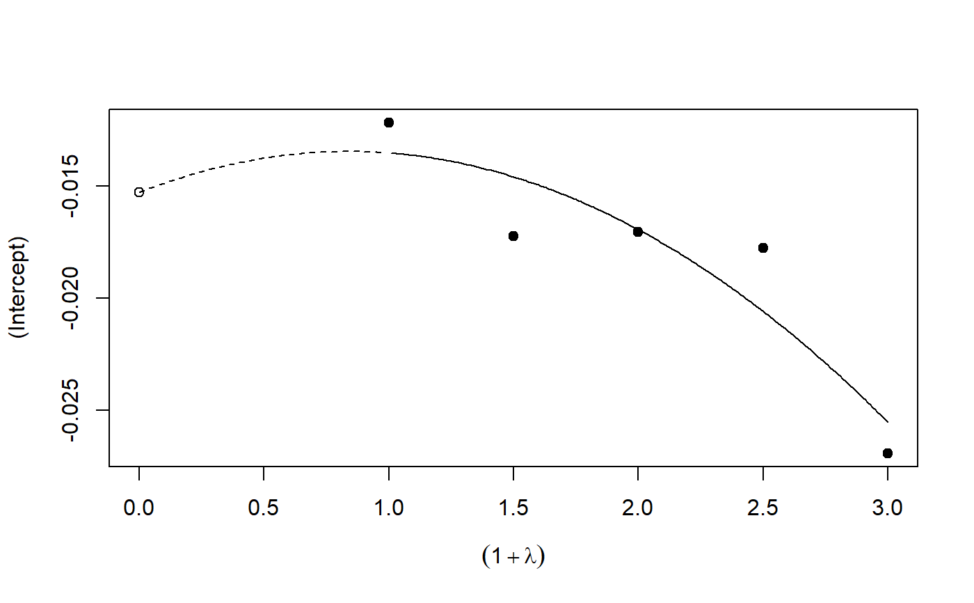
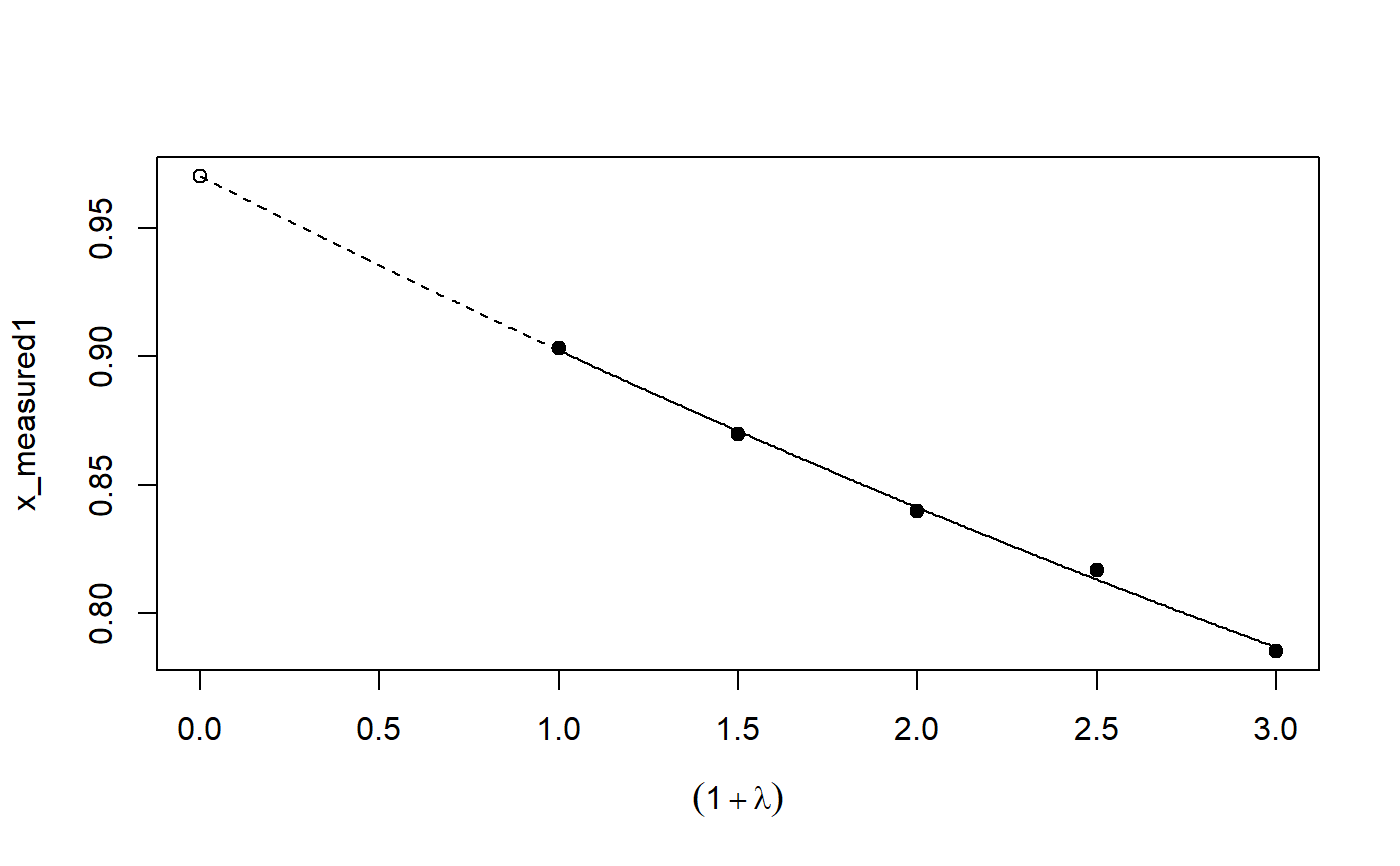
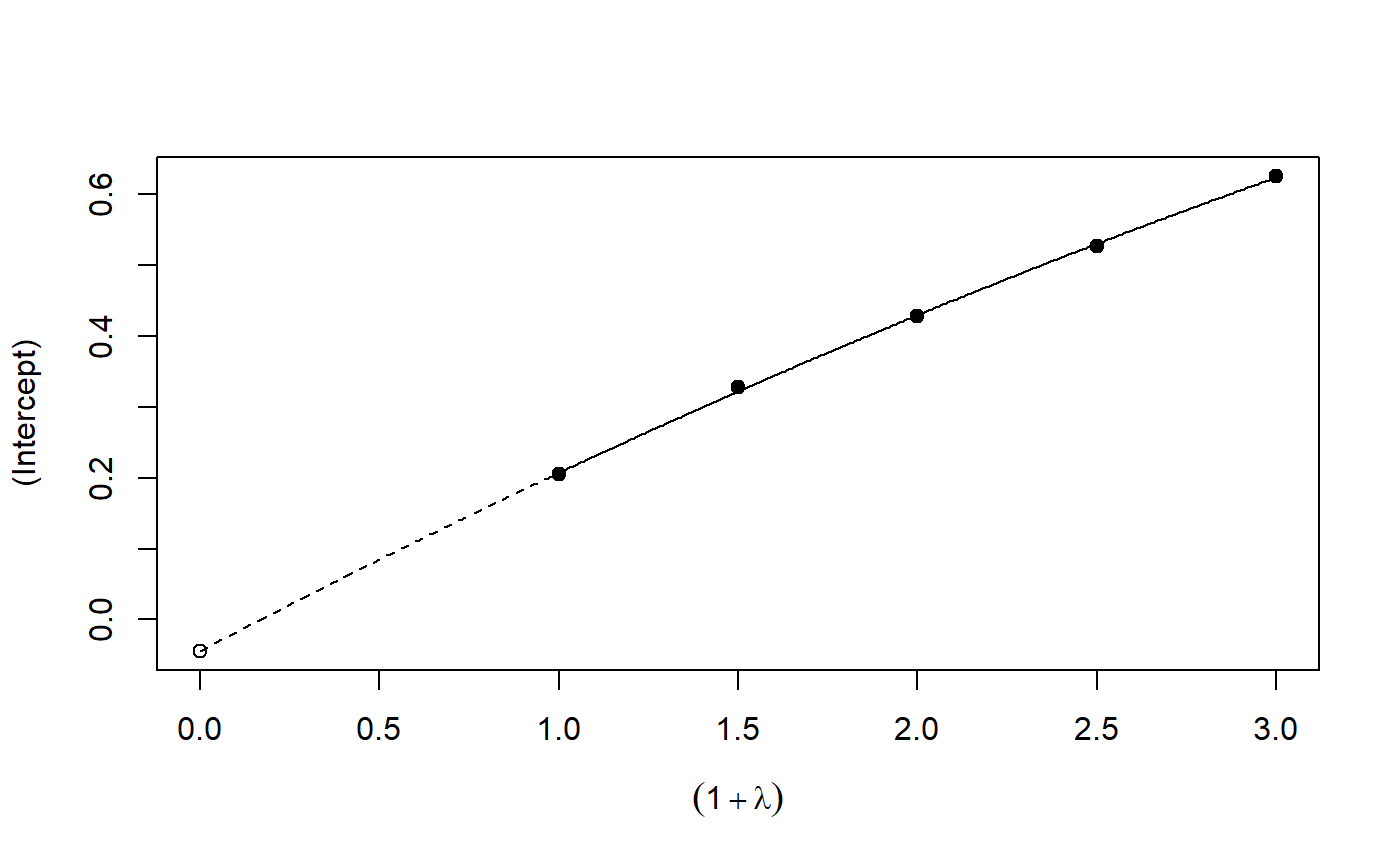
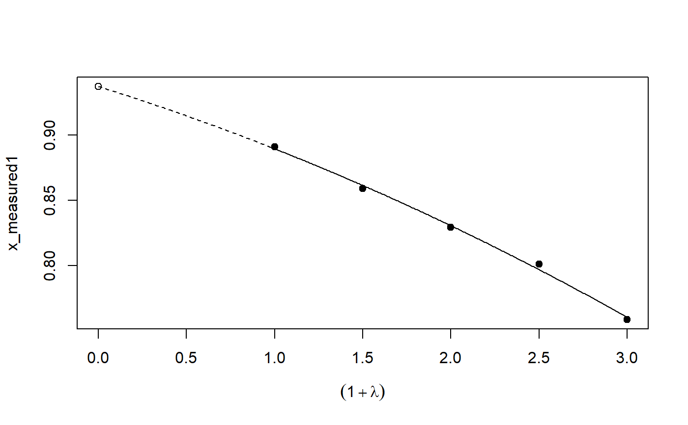
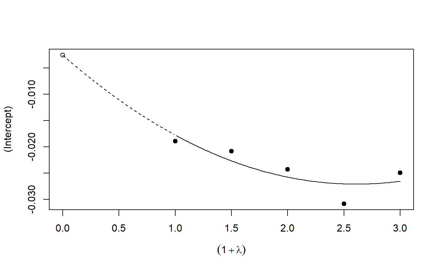
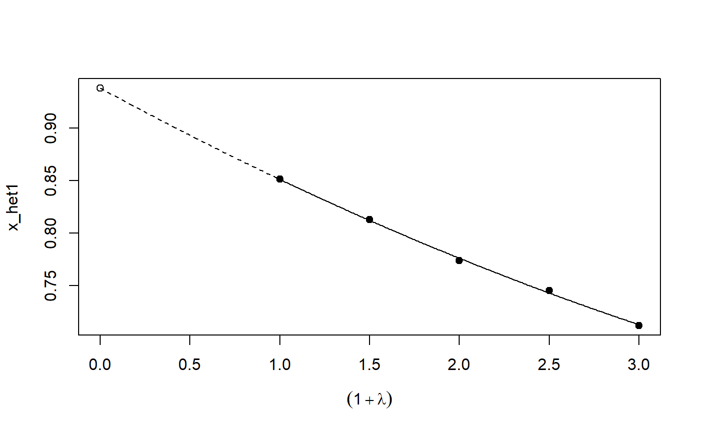
# See example(simex) and example(mcsimex)
## Seed
set.seed(49494)

## simulating the measurement error standard deviations
sd_me1 <- 0.3
sd_me2 <- 0.4
temp <- runif(100, min = 0, max = 0.6)
sd_me_het1 <- sort(temp)
temp2 <- rnorm(100, sd = 0.1)
sd_me_het2 <- abs(sd_me_het1 + temp2)

## simulating the independent variables x (real and with measurement error):
x_real1 <- rnorm(100)
x_real2 <- rpois(100, lambda = 2)
x_real3 <- -4*x_real1 + runif(100, min = -2, max = 2)  # correlated to x_real

x_measured1 <- x_real1 + sd_me1 * rnorm(100)
x_measured2 <- x_real2 + sd_me2 * rnorm(100)
x_het1 <- x_real1 + sd_me_het1 * rnorm(100)
x_het2 <- x_real3 + sd_me_het2 * rnorm(100)

## calculating dependent variable y:
y1  <- x_real1 + rnorm(100, sd = 0.05)
y2 <- x_real1 + 2*x_real2 + rnorm(100, sd = 0.08)
y3 <- x_real1 + 2*x_real3 + rnorm(100, sd = 0.08)


### one variable with homoscedastic measurement error
(model_real <- lm(y1  ~ x_real1))
#> 
#> Call:
#> lm(formula = y1 ~ x_real1)
#> 
#> Coefficients:
#> (Intercept)      x_real1  
#>   -0.004752     0.994554  
#> 

(model_naiv <- lm(y1  ~ x_measured1, x = TRUE))
#> 
#> Call:
#> lm(formula = y1 ~ x_measured1, x = TRUE)
#> 
#> Coefficients:
#> (Intercept)  x_measured1  
#>    -0.01217      0.90327  
#> 

(model_simex <- simex(model_naiv, SIMEXvariable = "x_measured1", measurement.error = sd_me1))
#> 
#> Naive model:
#> lm(formula = y1 ~ x_measured1, x = TRUE)
#> 
#> SIMEX-Variables: x_measured1
#> Number of Simulations: 100
#> 
#> Coefficients:
#> (Intercept)  x_measured1  
#>    -0.01528      0.97007  
#> 
plot(model_simex)


### two variables with homoscedastic measurement errors
(model_real2 <- lm(y2 ~ x_real1 + x_real2))
#> 
#> Call:
#> lm(formula = y2 ~ x_real1 + x_real2)
#> 
#> Coefficients:
#> (Intercept)      x_real1      x_real2  
#>    -0.01411      0.99094      2.00011  
#> 

(model_naiv2 <- lm(y2 ~ x_measured1 + x_measured2, x = TRUE))
#> 
#> Call:
#> lm(formula = y2 ~ x_measured1 + x_measured2, x = TRUE)
#> 
#> Coefficients:
#> (Intercept)  x_measured1  x_measured2  
#>      0.2050       0.8909       1.8593  
#> 

(model_simex2 <- simex(model_naiv2, SIMEXvariable = c("x_measured1", "x_measured2"),
                       measurement.error = cbind(sd_me1, sd_me2)))
#> 
#> Naive model:
#> lm(formula = y2 ~ x_measured1 + x_measured2, x = TRUE)
#> 
#> SIMEX-Variables: x_measured1, x_measured2
#> Number of Simulations: 100
#> 
#> Coefficients:
#> (Intercept)  x_measured1  x_measured2  
#>    -0.04414      0.93716      1.97311  
#> 

plot(model_simex2)


### one variable with increasing heteroscedastic measurement error
model_real
#> 
#> Call:
#> lm(formula = y1 ~ x_real1)
#> 
#> Coefficients:
#> (Intercept)      x_real1  
#>   -0.004752     0.994554  
#> 

(mod_naiv1 <- lm(y1  ~ x_het1, x = TRUE))
#> 
#> Call:
#> lm(formula = y1 ~ x_het1, x = TRUE)
#> 
#> Coefficients:
#> (Intercept)       x_het1  
#>     -0.0189       0.8513  
#> 

(mod_simex1 <- simex(mod_naiv1, SIMEXvariable = "x_het1",
     measurement.error = sd_me_het1, asymptotic = FALSE))
#> 
#> Naive model:
#> lm(formula = y1 ~ x_het1, x = TRUE)
#> 
#> SIMEX-Variables: x_het1
#> Number of Simulations: 100
#> 
#> Coefficients:
#> (Intercept)       x_het1  
#>   -0.002565     0.938262  
#> 

plot(mod_simex1)

# NOT RUN {
### two correlated variables with heteroscedastic measurement errors
(model_real3 <- lm(y3 ~ x_real1 + x_real3))

(mod_naiv2 <- lm(y3 ~ x_het1 + x_het2, x = TRUE))

(mod_simex2 <- simex(mod_naiv2, SIMEXvariable = c("x_het1", "x_het2"),
                     measurement.error = cbind(sd_me_het1, sd_me_het2), asymptotic = FALSE))
plot(mod_simex2)


### two variables, one with homoscedastic, one with heteroscedastic measurement error
model_real2

(mod_naiv3 <- lm(y2 ~ x_measured1 + x_het2, x = TRUE))

(mod_simex3 <- simex(mod_naiv3, SIMEXvariable = c("x_measured1", "x_het2"),
                     measurement.error = cbind(sd_me1, sd_me_het2), asymptotic = FALSE))


### glm: two variables, one with homoscedastic, one with heteroscedastic measurement error
t <- x_real1 + 2*x_real2
g <- 1 / (1 + exp(-t))
u <- runif(100)
ybin <- as.numeric(u < g)


(logit_real <- glm(ybin ~ x_real1 + x_real2, family = binomial))

(logit_naiv <- glm(ybin ~ x_measured1 + x_het2, x = TRUE, family = binomial))

(logit_simex <- simex(logit_naiv, SIMEXvariable = c("x_measured1", "x_het2"),
                      measurement.error = cbind(sd_me1, sd_me_het2), asymptotic = FALSE))
summary(logit_simex)
print(logit_simex)
plot(logit_simex)
# }

Error or misclassification correction in models using (MC)SIMEX

Details

References

See also

Examples

Contents

Author